Precificação de Opções

OPTION THEORY

In everyday conversation we often use the word “option” as synonymous with “choice” or “alternative”; thus we speak of someone as “having a number of options.” In finance option refers specifically to the opportunity to trade in the future on terms that are fixed today. Smart managers know that it is often worth paying today for the option to buy or sell an asset tomorrow.

Since options are so important, the financial manager needs to know how to value them. Finance experts always knew the relevant variables—the exercise price and the exercise date of the option, the risk of the underlying asset, and the rate of interest. But it was Black and Scholes who first showed how these can be put together in a usable formula.

The Black–Scholes formula was developed for simple call options and does not directly apply to the more complicated options often encountered in corporate finance. But Black and Scholes’s most basic ideas—for example, the risk-neutral valuation method implied by their formula—work even where the formula doesn’t.

Brealey, Myers and Allen,"Principles of Corporate Finance", 12th Ed., McGraw-Hill Education, 2017.

EXPLICAÇÃO DO RISK-NEUTRAL WORLD (NON-ARBITRAGE WORLD) E UM CÁLCULO DA PRECIFICAÇÃO DE BLACK-SCHOLES-MERTON

Isso tem que ficar bem claro!!! Black-Scholes-Merton é uma fórmula analítica fechada somente para precificação de "European stock options".

Temos que lembrar também das importantes suposições da Fórmula de Black-Scholes:

(a) Os retornos do preço do ativo subjacente segue um "lognormal random walk";

(b) Os "traders" de opções podem ajustar suas "posições" (ou, seu hedge) de forma contínua e sem custos significativos;

(d) O ativo subjacente não paga dividendos.

Because the Black–Scholes formula does not allow for early exercise, it cannot be used to value an American put exactly. But you can use the step-by-step binomial method as long as you check at each point whether the option is worth more dead than alive and then use the higher of the two values.

Brealey, Myers and Allen,"Principles of Corporate Finance", 12th Ed., McGraw-Hill Education, 2017.

THE GENERAL BINOMIAL METHOD

There is a neat little formula that relates the up and down changes to the standard deviation of stock returns:

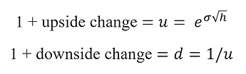
Where

e = base for natural logarithms = 2.718

σ = standard deviation of (continuously compounded) stock returns (%per annum)

h = interval as fraction of a year

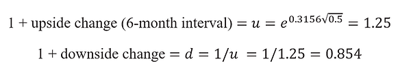
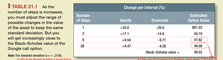
When we said that Google’s stock price could either rise by 25% or fall by 20% over six months (h = .5), our figures were consistent with a figure of 31.56% for the standard deviation of annual returns (To find the standard deviation given u, we turn the formula around: σ=log(u)/sqrt(h), where log = natural logarithm. In our example,σ=log(1.25)/sqrt(0.5)=0.3156).

To work out the equivalent upside and downside changes when we divide the period into two three-month intervals (h = .25), we use the same formula:

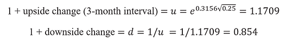
The center columns in Table 21.1 show the equivalent up and down moves in the value of the firm if we chop the period into six monthly or 26 weekly periods, and the final column shows the effect on the estimated option value.

Brealey, Myers and Allen,"Principles of Corporate Finance", 12th Ed., McGraw-Hill Education, 2017.

PRECIFICAÇÃO DE BLACK-SCHOLES-MERTON UTILIZANDO SIMULAÇÃO DE MONTE CARLO

The risk-neutral valuation principle states that a derivative can be valued by (a) calculating the expected payoff on the assumption that the expected return from the underlying asset equals the risk-free interest rate and (b) discounting the expected payoff at the risk-free interest rate.

When interest rates are constant, risk-neutral valuation provides a well-defined and unambiguous valuation tool. When interest rates are stochastic, it is less clear-cut. (texto introdutório do Capt. 28 - Martingales and Measures do Livro do John C. Hull, "Options and Other Derivatives").

******************************************************

When used to value an option, Monte Carlo simulation uses the risk-neutral valuation result. We sample paths to obtain the expected payoff in a risk-neutral world and then discount this payoff at the risk-free rate. Consider a derivative dependent on a single market variable S that provides a payoff at time T. Assuming that interest rates are constant, we can value the derivative as follows:

1. Sample a random path for S in a risk-neutral world.

2. Calculate the payoff from the derivative.

3. Repeat steps 1 and 2 to get many sample values of the payoff from the derivative in a risk-neutral world.

4. Calculate the mean of the sample payoffs to get an estimate of the expected payoff in a risk-neutral world.

5. Discount this expected payoff at the risk-free rate to get an estimate of the value of the derivative.

"Seção 21.6 - Monte Carlo Simulation", do "Chapter 21. - Basic Numerical Procedures", do livro do John C. Hull, “Options, Futures, and Other Derivatives”, 10th Edition, Publisher: Pearson, 2018.

THE KEY ADVANTAGE OF MONTE CARLO SIMULATION

The key advantage of Monte Carlo simulation is that it can be used when the payoff depends on the path followed by the underlying variable S as well as when it depends only on the final value of S. (For example, it can be used when payoffs depend on the average value of S between time 0 and time T.) Payoffs can occur at several times during the life of the derivative rather than all at the end. Any stochastic process for S can be accommodated. As will be shown shortly, the procedure can also be extended to accommodate situations where the payoff from the derivative depends on several underlying market variables. The drawbacks of Monte Carlo simulation are that it is computationally very time consuming and cannot easily handle situations where there are early exercise opportunities.14

14 - As discussed in Chapter 27, a number of researchers have suggested ways Monte Carlo simulation can be extended to value American options

Monte Carlo simulation tends to be numerically more efficient than other procedures when there are three or more stochastic variables. This is because the time taken to carry out a Monte Carlo simulation increases approximately linearly with the number of variables, whereas the time taken for most other procedures increases exponentially with the number of variables. One advantage of Monte Carlo simulation is that it can provide a standard error for the estimates that it makes. Another is that it is an approach that can accommodate complex payoffs and complex stochastic processes. Also, it can be used when the payoff depends on some function of the whole path followed by a variable, not just its terminal value.

THE RISK OF AN OPTION

How risky is the Google call option? We have seen that you can exactly replicate a call by a combination of risk-free borrowing and an investment in the stock. So the risk of the option must be the same as the risk of this replicating portfolio. We know that the beta of any portfolio is simply a weighted average of the betas of the separate holdings. So the risk of the option is just a weighted average of the betas of the investments in the loan and the stock.

On past evidence the beta of Google stock is βstock = 1.15; the beta of a risk-free loan is βloan = 0. You are investing $297.89 in the stock and –$248.36 in the loan. (Notice that the investment in the loan is negative—you are borrowing money.) Therefore the beta of the option is βoption = (–248.36 × 0 + 297.89 × 1.15)/(–248.36 + 297.89) = 6.92 [βoption = 6.92].

Notice that, because a call option is equivalent to a levered position in the stock, it is always riskier than the stock itself. In Google’s case the option is nearly seven times as risky as the stock. As time passes and the price of Google stock changes, the risk of the option will also change.

Brealey, Myers and Allen,"Principles of Corporate Finance", 12th Ed., McGraw-Hill Education, 2017.

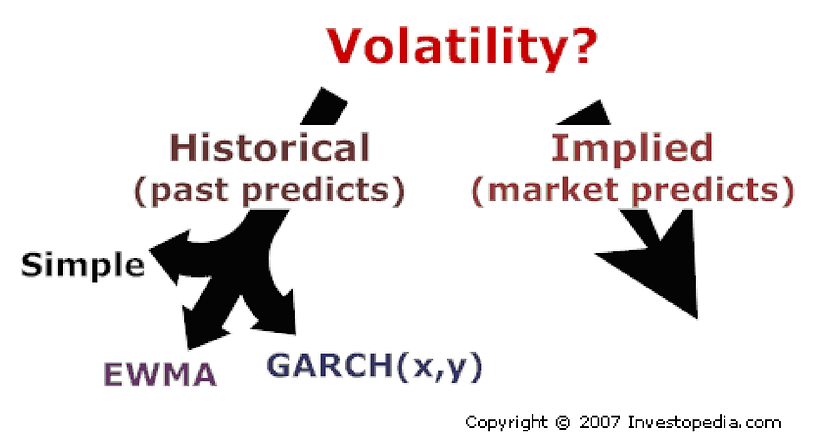
CALCULATING IMPLIED VOLATILITIES

So far we have used our option pricing model to calculate the value of an option given the standard deviation of the asset’s returns. Sometimes it is useful to turn the problem around and ask what the option price is telling us about the asset’s volatility

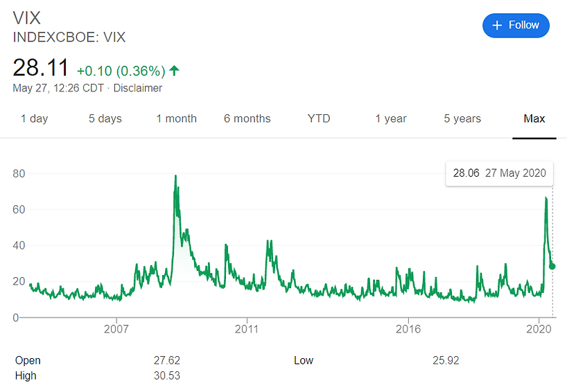
The Chicago Board Options Exchange (CBOE) regularly publishes the implied volatility on the Standard and Poor’s index, which it terms “the VIX”.

The Market Volatility Index or VIX measures the volatility that is implied by near-term Standard & Poor’s 500 Index options and is therefore an estimate of expected future market volatility over the next 30 calendar days. Implied market volatilities have been calculated by the Chicago Board Options Exchange (CBOE) since January 1986, though in its current form the VIX dates back only to 2003.

Investors regularly trade volatility. They do so by buying or selling VIX futures and options contracts. Since these were introduced by the Chicago Board Options Exchange (CBOE), combined trading activity in the two contracts has grown to more than 100,000 contracts per day, making them two of the most successful innovations ever introduced by the exchange.

Brealey, Myers and Allen,"Principles of Corporate Finance", 12th Ed., McGraw-Hill Education, 2017.